Issue 001 Autumn 2025

From a Tennis Bottle Challenge to the Poisson Distribution

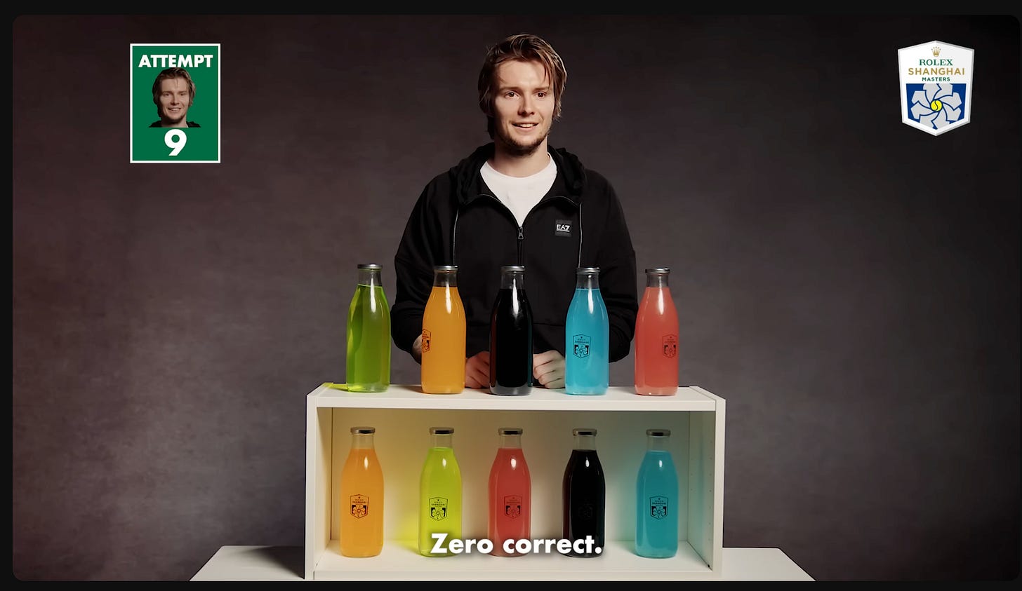
TennisTV’s “Bottle Challenge” at the Shanghai Masters

TennisTV, in some underrated Shanghai Masters promo content, had professional players attempt a “bottle challenge”. Five bottles of different colors are lined up in front of you. The same five colors are hidden below them in some unknown order. Your job is simple: match each top bottle with the identically colored one beneath it. After every move, usually swapping two bottles, you’re told how many positions are currently correct.

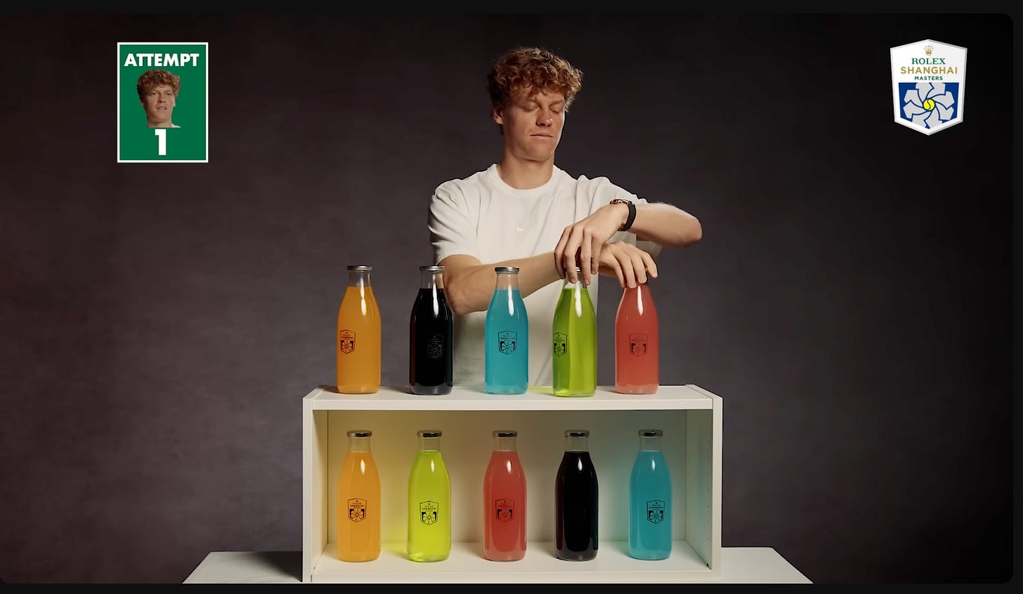
Hilarity ensues as competitive tennis players take their…unique...approaches to this game. Some solve it in five swaps; others take more than 15. Bublik, in particular, cannot believe how often he hears “zero correct.”

It made me wonder: how common is “zero correct”?

Translating to Permutations

Let’s translate this into mathematical language. Label the correct hidden order as 1-5. Then the top row is a reordering of those numbers. For example, (2, 4, 3, 1, 5), where 3 and 5 are in their “correct” positions. This is a permutation: an ordering of the numbers. You can also say a permutation of n elements (n=5 here) is a mapping of 1…n onto itself. Explicitly, our mapping above is 1 → 2, 2 → 4, 3 → 3, 4 → 1, 5 → 5.

In this language, the number of “correct” bottles is the number of fixed points of the mapping; the indices i where i → i. There are n! permutations total, so the natural question is: “how many of these have zero fixed points”?

Empirically, let’s run a simple Python script that does this. This will quickly get too large to compute, but we can run it for n=1 to n=10:

karan:~/projects/scratch$ python permutation_analysis.py --zero-fixed-only -m 10 --include-percent
Permutation Fixed Point Analysis
============================================================

Zero fixed point permutations for n = 1 to 10:

 n |    zero | percent
----------------------
 1 |       0 |    0.00%
 2 |       1 |   50.00%
 3 |       2 |   33.33%
 4 |       9 |   37.50%
 5 |      44 |   36.67%
 6 |     265 |   36.81%
 7 |    1854 |   36.79%
 8 |   14833 |   36.79%
 9 |  133496 |   36.79%
10 | 1334961 |   36.79%

Interestingly, the percentage of “zero correct” permutations converges to ~36.79%. Why?

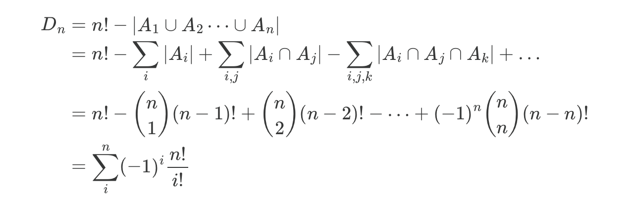
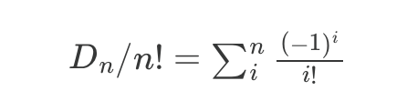
Counting Derangements

Permutations with no fixed points have a name: derangements.. To compute this, we can take the total number of permutations and subtract those with a fixed point. Let Aᵢ be the set of permutations with element i fixed. We want the size of the union | A₁ ∪ A₂ … ∪ Aₙ | so we can compute n! - | A₁ ∪ A₂ … ∪ Aₙ |. We can use the Principle of Inclusion-Exclusion to sum the union on the right side

In other words, the number of derangements of n Dₙ is:

For more information about the Principle of Inclusion / Exclusion or to understand the steps in the equation above, you can interrogate this Claude chat.

36.79%

Now we can answer the question: “why 36.79%”?

The percentage of derangements (“zero correct”) over the total number of permutations is

Using the Taylor series definition of eˣ, we can see that

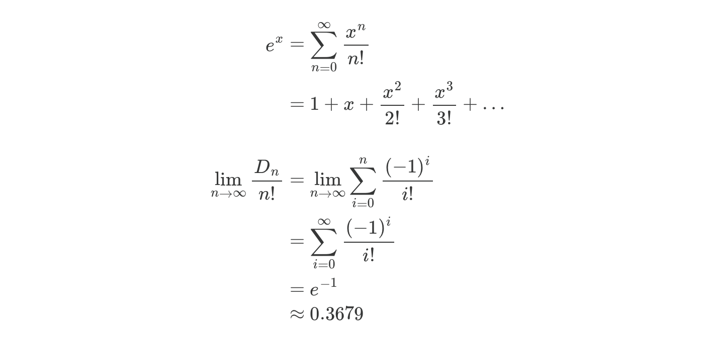
So we got the answer to our 36.79%! Surprise, it involves e!

The other fixed points

The number of derangements also gives us a way to calculate the number of permutations of n with exactly k fixed points. Choosing k elements to fix and multiplying by the number of ways to arrange (derange?) the rest,

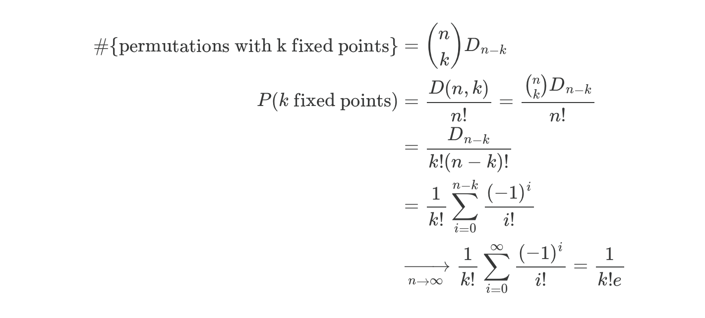
Using the script from earlier, we can confirm for n = 8, 9, 10:

k  |           8                9                 10
-----------------------------------------------------------
0  |   14833 (36.79%)   133496 (36.79%)    1334961 (36.79%)
1  |   14832 (36.79%)   133497 (36.79%)    1334960 (36.79%)
2  |    7420 (18.40%)    66744 (18.39%)     667485 (18.39%)
3  |    2464 (6.11%)     22260 (6.13%)      222480 (6.13%)
4  |     630 (1.56%)      5544 (1.53%)       55650 (1.53%)
5  |     112 (0.28%)      1134 (0.31%)       11088 (0.31%)
6  |      28 (0.07%)       168 (0.05%)        1890 (0.05%)
7  |       0 (0.00%)        36 (0.01%)         240 (0.01%)
8  |       1 (0.00%)         0 (0.00%)          45 (0.00%)
9  |         -               1 (0.00%)           0 (0.00%)
10 |         -                 -                 1 (0.00%)

For our original question: we’ve shown it’s really common (70%+) to get zero or one fixed point in a random permutation! Moreover, this stays stable no matter how large n gets.

You promised me Poisson

OK, fair. A Poisson process is one where:

Events occur independently
The average rate of occurrence is constant
Two events cannot occur at exactly the same instant

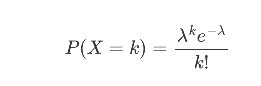
Common examples: number of emails per hour, radioactive decays per second, typos per page. The Poisson distribution counts those events. It has a single parameter λ, the expected number of events in an interval. The probability of exactly k events is:

However, a Poisson distribution is more general than it first seems: it can count the total of random variables with rare, independent “successes” with a fixed expected value λ. As the value of n gets larger, the probability of any index i being a fixed point gets closer to independent. That is, we can start ignoring where other indices are placed when considering our index because there are so many “slots”. Also, with expected value linearity, we can always ignore independence.

Substituting for λ the expected number of fixed points, which in this case is E[fixed points] = P(any given point being fixed) * n = 1/n * n = 1, the Poisson and derangement formulas converge! In other words, probability of a permutation with k fixed points converges to the Poisson distribution.

You can confirm for yourself that the values in the table above for n = 8, 9, 10 roughly match the formula above for the Poisson distribution! Pretty cool.